Topics

Stability

The stability of a general dynamical system with no input can be described with Lyapunov stability criteria.

• A linear system is called bounded-input bounded-output (BIBO) stable if its output will stay bounded for any bounded input.
• Stability for nonlinear systems that take an input is input-to-state stability (ISS), which combines Lyapunov stability and a notion similar to BIBO stability.

For simplicity, the following descriptions focus on continuous-time and discrete-time linear systems.

Mathematically, this means that for a causal linear system to be stable all of the poles of its transfer function must have negative-real values, i.e. the real part of each pole must be less than zero. Practically speaking, stability requires that the transfer function complex poles reside

• in the open left half of the complex plane for continuous time, when the Laplace transform is used to obtain the transfer function.
• inside the unit circle for discrete time, when the Z-transform is used.

The difference between the two cases is simply due to the traditional method of plotting continuous time versus discrete time transfer functions. The continuous Laplace transform is in Cartesian coordinates where the ${\displaystyle x}$ axis is the real axis and the discrete Z-transform is in circular coordinates where the ${\displaystyle \rho }$ axis is the real axis.

When the appropriate conditions above are satisfied a system is said to be asymptotically stable; the variables of an asymptotically stable control system always decrease from their initial value and do not show permanent oscillations. Permanent oscillations occur when a pole has a real part exactly equal to zero (in the continuous time case) or a modulus equal to one (in the discrete time case). If a simply stable system response neither decays nor grows over time, and has no oscillations, it is marginally stable; in this case the system transfer function has non-repeated poles at complex plane origin (i.e. their real and complex component is zero in the continuous time case). Oscillations are present when poles with real part equal to zero have an imaginary part not equal to zero.

If a system in question has an impulse response of

${\displaystyle \ x[n]=0.5^{n}u[n]}$

then the Z-transform (see this example), is given by

${\displaystyle \ X(z)={\frac {1}{1-0.5z^{-1}}}\ }$

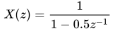
which has a pole in ${\displaystyle z=0.5}$ (zero imaginary part). This system is BIBO (asymptotically) stable since the pole is inside the unit circle.

However, if the impulse response was

${\displaystyle \ x[n]=1.5^{n}u[n]}$

then the Z-transform is

${\displaystyle \ X(z)={\frac {1}{1-1.5z^{-1}}}\ }$

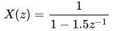
which has a pole at ${\displaystyle z=1.5}$ and is not BIBO stable since the pole has a modulus strictly greater than one.

Numerous tools exist for the analysis of the poles of a system. These include graphical systems like the root locus, Bode plots or the Nyquist plots.

Mechanical changes can make equipment (and control systems) more stable. Sailors add ballast to improve the stability of ships. Cruise ships use antiroll fins that extend transversely from the side of the ship for perhaps 30 feet (10 m) and are continuously rotated about their axes to develop forces that oppose the roll.

Controllability and observability

Controllability and observability are main issues in the analysis of a system before deciding the best control strategy to be applied, or whether it is even possible to control or stabilize the system. Controllability is related to the possibility of forcing the system into a particular state by using an appropriate control signal. If a state is not controllable, then no signal will ever be able to control the state. If a state is not controllable, but its dynamics are stable, then the state is termed stabilizable. Observability instead is related to the possibility of observing, through output measurements, the state of a system. If a state is not observable, the controller will never be able to determine the behaviour of an unobservable state and hence cannot use it to stabilize the system. However, similar to the stabilizability condition above, if a state cannot be observed it might still be detectable.

From a geometrical point of view, looking at the states of each variable of the system to be controlled, every "bad" state of these variables must be controllable and observable to ensure a good behaviour in the closed-loop system. That is, if one of the eigenvalues of the system is not both controllable and observable, this part of the dynamics will remain untouched in the closed-loop system. If such an eigenvalue is not stable, the dynamics of this eigenvalue will be present in the closed-loop system which therefore will be unstable. Unobservable poles are not present in the transfer function realization of a state-space representation, which is why sometimes the latter is preferred in dynamical systems analysis.

Solutions to problems of uncontrollable or unobservable system include adding actuators and sensors.